Fast but False Progress on Benchmarks with Richer Feedback
Stanford University
Detailed benchmark scores help developers pinpoint the weaknesses of complex models. We show this feedback can accelerate ranking and score inflation on HELM1, LiveBench, Open LLM, SWE-bench, and Terminal-Bench-Science. In as few as 2 submissions, we manufacture a leaderboard winner that falls behind on unseen data. It is open whether past evidence of reliable ordinary benchmark reuse with scalar feedback holds with richer feedback.
Code repositoryTheory paperTechnical report (soon)
1. Alphabetically ordered benchmark names. ↩
0. Richer feedback
Benchmarks are a standard way to compare machine learning systems and guide model selection. For these comparisons to inform deployment, they must generalize: performance on the underlying test set should reflect performance on fresh data from the same population.
An aggregate benchmark score summarizes a model’s performance in one number. Many leaderboards also publish a separate score per criterion or task. We call this breakdown rich feedback.
This is an increasingly relevant type of evaluation in modern AI development. Indeed, general-purpose models can do many different tasks, and developers need to know where they work well and where they fail—a motivation behind benchmarks like HELM. A single aggregate can hide those differences and obscure what is being measured (Burnell et al., 2023; Jiang et al., 2026). This is especially relevant when test examples are private, as in ARC-AGI and other evaluations that use private data to reduce contamination risks.2 This creates the tension we focus on: evaluating more criteria gives developers a fuller picture, but returning more scores can also leak more information about the test set with each submission, making it easier to overfit through repeated use.
2. Examples include Vals AI’s proprietary benchmarks and Scale’s SWE-Bench Pro private commercial subset. ↩
The tables below give examples of rich feedback. Each row is a model or agent configuration, and each task or domain column summarizes its performance on a different set of examples.
Scroll to see all domain scores.
| Model | Aggregate score | Earth sciences | Engineering sciences | Life sciences | Mathematical sciences | Physical sciences |
|---|---|---|---|---|---|---|
| GPT-6 AstraCodex · max effort | 68.1 | 79.2 | 70.4 | 59.6 | 80.4 | 58.8 |
| Opus 5.5Claude Code · max effort | 63.3 | 62.5 | 63.0 | 54.4 | 76.5 | 60.8 |
GPT-6 Astra has the higher aggregate score in this excerpt; Opus 5.5 scores higher on physical sciences.
Scroll to see all task scores.
| Model | Aggregate score | MMLU-ProKnowledge | GPQAScience | IFEvalInstructions | WildBenchOpen-ended tasks | Omni-MATHMathematics |
|---|---|---|---|---|---|---|
| Claude 3.5 Sonnet | 65.3 | 77.7 | 56.5 | 85.6 | 79.2 | 27.6 |
| GPT-4o | 63.4 | 71.3 | 52.0 | 81.7 | 82.8 | 29.3 |
Claude 3.5 Sonnet has the higher aggregate score in this excerpt; GPT-4o scores higher on open-ended tasks and mathematics.
Based on the benchmarks we study below, each leaderboard submission receives the following scores:
- HELM Capabilities (v1.15.0): the five task scores shown above.
- HELM Lite (v1.13.0): ten scores, covering question answering, mathematics, and translation.
- LiveBench (2024-10-22 snapshot): 18 task scores, including code completion, spatial reasoning, combining tables, and summarization.
- Open LLM (v2): six task scores: IFEval, BBH, MATH Lvl 5, GPQA, MuSR, and MMLU-Pro.
- SWE-bench Verified (2026-09-21 snapshot): ten repository-group scores reconstructed from released per-instance results. Repositories with fewer than ten instances are pooled.
- Terminal-Bench-Science (v0.1): five domain scores reconstructed from released task outcomes: earth, engineering, life, mathematical, and physical sciences.
Every new submission returns another set of scores. Repeating this process on the same examples gives an attacker information that can be used to inflate apparent progress, in both scores and model selection. Our goal is to quantify the extent of this vulnerability using the modern benchmark data above. Note that the benchmarks above are not meant to be private and give per-item scores, so we instead simulate an interface where the attacker only sees task/criterion aggregates. The point is to show that, even without knowing the test set or anything about the benchmark in general, one can easily beat all other models in terms of aggregate score.
To approximate the performance on unseen data, we randomly split each benchmark into a reused set that returns leaderboard submission feedback and a held-out set reserved for evaluation. We then follow the reused-set ranking and scores before and after adding the attack, and compare the two choices on held-out data. We do so over 250 trials by default, over the randomness of the splits.
For starters, we will overview the main results quantifying the vulnerability, ignoring for the moment which attack allowed obtaining them.
Snapshot sources and score reconstruction
The data provenance notes identify the retained benchmark snapshots and explain how the introductory score tables are reconstructed from their public records.
1. Best-model selection
Does the best-ranked model hold up on unseen data?
We measure model selection loss: the held-out score of the model chosen before the attack minus that of the model chosen afterward. Positive values mean following the new ranking made selection worse.
Below, we observe that following the public ranking lowers held-out performance on all six benchmarks at 128 leaderboard submissions. In fact, in all cases, 16 submissions suffice to approach the 1 pp loss mark. The largest losses are on LiveBench and HELM Lite.

Each submission budget produces its own final attack model, so its held-out performance can improve as well as deteriorate. The dip for Terminal-Bench-Science reflects such an improvement; selection loss stays positive because the new choice still performs worse, on average, than the original public winner.
Selected-model scores, rank changes and budgets
| Benchmark | No attack (%) | With attack (%) | Loss (pp) [95% interval] | Rank drop [95% interval] |
|---|---|---|---|---|
| LiveBench | 60.41 | 55.82 | 4.59 [4.26, 4.93] | +2.36 [+2.13, +2.60] |
| HELM Capabilities | 81.46 | 80.53 | 0.93 [0.82, 1.04] | +2.44 [+2.16, +2.71] |
| HELM Lite | 74.12 | 69.32 | 4.80 [4.61, 4.97] | +3.64 [+3.52, +3.75] |
| Open LLM | 47.71 | 45.31 | 2.40 [2.24, 2.58] | +2.80 [+2.64, +2.96] |
| SWE-bench Verified | 77.71 | 76.65 | 1.07 [0.78, 1.34] | +3.08 [+2.06, +4.07] |
| Terminal-Bench-Science | 65.81 | 62.78 | 3.04 [2.36, 3.77] | +0.80 [+0.65, +0.95] |
| Benchmark | Reused (%) | Held out (%) |
|---|---|---|
| LiveBench | 60.70 | 60.41 |
| HELM Capabilities | 82.01 | 81.46 |
| HELM Lite | 74.20 | 74.12 |
| Open LLM | 48.13 | 47.71 |
| SWE-bench Verified | 80.44 | 77.71 |
| Terminal-Bench-Science | 69.76 | 65.75 |
The comparison pool contains the original models and the final router, excluding intermediate candidates. Selection ties favor an original model, then lexical order; evaluation ties share rank. HELM Lite selects and ranks by mean win rate, while its score loss uses the equal-category mean. Other score scales follow the original evaluators.
The intervals describe variation across splits of these snapshots; they do not account for a change in the underlying data. See the metric definitions and complete results for all budgets and paired trials.
False winners and a counterexample
A false winner ranks first on the reused set but not on the held-out set. The curves below show the fraction of trials whose final attack model is a false winner, with additional curves requiring a held-out score at least 1, 2, or 5 pp below the best original model. This is the held-out score gap to the best original model; selection loss instead compares the public-selected models before and after the attack.

These rates describe the final model at each budget, so they need not keep rising. A model can remain first publicly while improving held out, so fewer trials exceed a score-gap threshold or count as false winners.
The first tested submission counts reaching a 90% false-winner rate are LiveBench, 4; HELM Capabilities, 16; HELM Lite, 64; Open LLM, 16; SWE-bench Verified, 2; Terminal-Bench-Science, 8. Intermediate counts were not tested. The false-winner rates and intervals include every tested budget.
A counterexample: Terminal-Bench
In an attempt to also replay Terminal-Bench 4.0, selection improves by 1.52 pp at 128 submissions, despite 77.2% false winners. This can happen as the original public winner need not be the best held-out model. Replacing it with a model between those two in held-out performance improves selection, even though the replacement is still a false winner. This illustrates why false-winner frequency alone does not measure selection harm.
The best-score generalization gap nevertheless exceeds its no-attack baseline. Improving the chosen model does not ensure that its public score is reliable: the best public and held-out scores can move farther apart while the selected model gets better. See the counterexample’s data and methods for the full replay.
2. Best-score generalization
Does the best score found through repeated submissions hold up on unseen data?
Now after each leaderboard submission, we compare the best score so far on the reused set with the best score so far on the held-out set. The largest absolute gap over this history is the score generalization gap. The two best scores may belong to different models. The baseline uses only the original benchmark models; it can be positive because their scores already differ between the two splits.
Below, we observe that the gap grows early on LiveBench and SWE-bench Verified, while HELM Lite and Open LLM continue to diverge with more submissions. Recall that these curves tell us how well the best reported score holds up; Figure 1 shows what happens to the model we choose.

Each budget ends with its own final attack model, so the final model from a shorter run is absent from the longer run’s history. The maximum is taken within each of these histories, so the plotted gap can decrease across budgets even though a running maximum cannot decrease within one run.
Metric, uncertainty and complete results
Let  denote the reused set and
 the held-out set. Write
 for the smallest loss on set
 among the first
 submissions, where loss is one minus the score on a 0–1 scale. With
 original models and
 new submissions,

The history includes the original models and all new submissions, including the final one. Scores follow each benchmark’s evaluator; HELM Lite uses equal-category means and SWE-bench Verified weights instances equally. We compare attack and baseline errors on the same trials and resample those pairs to form confidence bounds. Statistical details.
The complete score-gap curves include all budgets and intervals.
3. How the attack works
To keep things simple and to avoid running expensive model inferences, each attack leaderboard submission is a router: a rule that sends each prompt to one of two existing models. The attack uses public task scores from repeated submissions to choose which model handles each prompt. We illustrate the steps with one selected HELM Lite trial using 32 leaderboard submissions. The attack is mostly an adaptation of the boosting attack, which we discuss at the end of the section.
A. Choosing the two routing endpoints
The two models should be strong, but different enough that routing between them can help. We first remove models for which another model does at least as well on every task and better on at least one. Among the five highest-ranked models left, we choose the pair with the largest average absolute difference between their task scores.
In this example trial, that gives us A: Gemma 2 27B IT and B: DeepSeek V3. Before any new submissions, GPT-4o (August 2024) leads the public ranking.
B. Turning task scores into weights
Each submission is simply an independent random routing rule to choose model A or B for each prompt. Only a hash of the input/prompt is required to make the choice repeatable, so identical prompts always go to the same model. These rules are fixed before any feedback arrives. Each submission returns ten category scores in this example; two are shown below.
| Submission | LegalBench (%) | MMLU (%) |
|---|---|---|
| A | 72.73 | 66.81 |
| B | 70.46 | 81.33 |
| Candidate 1 | 70.17 | 74.81 |
| Candidate 2 | 70.20 | 73.26 |
| Candidate 3 | 70.50 | 75.56 |
For a given task  , let
 be the two models’ public losses, where loss is one minus the score on a 0–1 scale. Their average is the reference loss for random routing. If candidate returns public loss
 , we give it the following weight:
Weight = reference loss − candidate loss
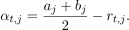 (1)
A candidate that beats the reference gets a positive weight; a candidate that does worse gets a negative weight. The farther its loss is from the reference, the more its choices count. In the example, candidate 1’s LegalBench feedback gives weight -0.01426.
C. Combining the routing choices
For prompt  , write
 for candidate ’s choice: +1 selects
 and −1 selects
 . Add these choices with their task-specific weights:
Final choice = sign of the weighted sum
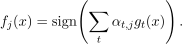 (2)
The final router selects when  and when
 . Thus, a positive weight supports a candidate’s choice; a negative weight reverses it. Each task score weakly reflects which choices worked on that task. Combining many such scores strengthens the signal on the reused examples. For the reused LegalBench prompt with the smallest public hash, the weighted vote is +0.02201, so the final router chooses A.
The final router takes first place publicly but ranks fifth on the held-out split. Following it instead of GPT-4o lowers held-out performance from 74.10% to 70.14%, a 3.95 pp model-selection loss. This example illustrates the mechanism only; the earlier curves include every trial.

DeepSeek V3 has a slightly higher public mean score than GPT-4o in this figure, yet GPT-4o leads the original ranking. HELM Lite ranks models by their average win rate against other models within categories, which can order them differently from these mean scores.
Our work builds on the elegant line of research on adaptive data analysis, initiated by Dwork et al. (2015), discussed further in our previous paper. The attack draws on Blum and Hardt’s boosting construction (2015), Hardt’s generalized wacky boosting (2015), and the feedback-weighted aggregation of Feldman, Frostig, and Hardt (2019). Here, an important adaptation is that we select two strong models with contrasting strengths by maximizing task-profile separation among the top five models on the public Pareto frontier. We then combine random routers using public task scores, with the specific aim of studying how feedback richness accelerates overfitting and affects model selection across modern benchmark snapshots.
4. Controlling feedback richness
How much does richer feedback make the attack more efficient?
We want to understand how much the number of evaluation criteria accelerates the inflations we found. Consider LiveBench as an example where richer feedback brings selection harm fast. At 8 leaderboard submissions, mean selection loss is 1.43 pp with 1 returned score and 4.29 pp with 18.
We group the 18 LiveBench tasks into a varying number of super-categories, and return one average score per group, keeping the model pairs, random routing rules, and evaluation fixed. Each outcome is plotted against submissions and the total number of scores released.
Below to the right, indexing by the total number of released scores brings the curves quite close. This suggests that the amount of feedback---simply defined as the total number of unit measurements---helps explain how quickly the attack succeeds. By 128 submissions, mean loss is 4.59–4.85 pp across all six interfaces. Coarser feedback delays harm here, at the cost of hiding task differences that may matter for model selection.

Details of controlled comparison and extension to false-winner rates

The submission counts needed for a 90% false-winner rate show a 16× spread. The corresponding totals of released scores vary by only 1.5×.
We use the same splits, models, model pairs, and random routing rules throughout. We divide the 18 tasks into equal-sized groups, chosen without looking at scores, and release 1, 2, 3, 6, 9, or 18 group averages. The attack combines routing choices separately for each group. Model pairs are chosen using all 18 public task scores and stay fixed.
With one released score, all tasks are averaged equally. With six scores, the groups are chosen independently of the scores. Both differ from the historical interface, which grouped tasks by subject.
The one-score and 18-score interfaces are unchanged by regrouping, so their range bars collapse. This indicates agreement across groupings; uncertainty across benchmark splits remains.
Scroll for all threshold values.
| Scores per candidate | 90% false-winner rate | Score generalization gap: +1 pp | Score generalization gap: +2 pp | |||
|---|---|---|---|---|---|---|
| Submissions | Coordinates | Submissions | Coordinates | Submissions | Coordinates | |
| 1 | 64 | 63 | 64 | 63 | 128 | 127 |
| 2 | 32 | 62 | 32 | 62 | 64 | 126 |
| 3 | 16 | 45 | 16 | 45 | 32 | 93 |
| 6 | 8 | 42 | 8 | 42 | 16 | 90 |
| 9 | 8 | 63 | 8 | 63 | 16 | 135 |
| 18 | 4 | 54 | 4 | 54 | 8 | 126 |
At equal totals of released score coordinates, the score-gap curves are close but do not coincide. Differences are at most 0.31 pp; 3 of 6 paired 95% intervals exclude zero.
The controlled-study methods describe the grouping protocol, complete results and reproduction steps.
Practical feedback policies: tasks, categories or one score
Now, let us think end-to-end about whether we can coarsen feedback to make it harder for the attacker to succeed. In particular, what if the attacker also has to choose its two models from the restricted feedback? A separate LiveBench comparison tests that question using 18 task scores, six natural category scores, or one overall score. The splits, seeds and submission budgets stay paired. Unlike the controlled study above, this changes both endpoint selection and the feedback used to build the router.
| Feedback | False winners at 16 | Selection loss at 128 (pp) |
|---|---|---|
| 18 task scores | 98.4% | +4.48 |
| 6 category scores | 99.2% | +4.84 |
| 1 overall score | 71.6% | +4.03 |
Returning only the overall score delays false winners here; six category scores offer no consistent improvement over task scores. Selection loss is half a percentage point better when releasing one aggregate score only. Yet, by 128 submissions, all three policies produce false winners in at least 99% of trials and lead to worse model selection. Thus, none establishes a safe policy. A more principled defense is described in our previous paper.
The feedback-policy study gives the paired protocol, selection losses and intervals.
5. Frequently asked questions
What information can the attacker see?
Only public task scores, task identity, and a stable prompt identifier are needed for routing. We use a prompt hash so identical prompts receive the same choice. Individual item inputs/prompts and scores remain hidden.
How do these attacks relate to ordinary model development?
This is an open question; these experiments measure vulnerability to deliberate attacks. Back in classical machine learning days, Roelofs et al. (2019) found little evidence of substantial overfitting across more than 100 Kaggle competitions. One explanation for reliable reuse is that developers mainly respond to clear improvements over the previous best, as in Blum and Hardt’s Ladder mechanism. Our accompanying theory paper shows fundamentally why this protection can weaken when models compete under different weightings of the criteria. Reassuring experience with scalar leaderboards therefore need not carry over to richer feedback.
The commercial stakes of LLM rankings also give developers incentives to game evaluation (Singh et al., 2025). Understanding how often the vulnerability studied here arises in ordinary development seems non-trivial, as we need to trace which criteria matter more in guiding later models and check whether the resulting gains persist on fresh data from the same population.
Can feedback counts predict vulnerability on another benchmark?
Not reliably. We tried on LiveBench and found that accounting for both released scores and reused examples aligns the score-gap curves well. But a fit learned there misestimates the submission count needed on the other benchmarks, so it cannot yet serve as a general vulnerability predictor. The prediction methods and results compare the fitted and observed thresholds.
Do repeated submissions add more than static task routing?
Yes. A static router sends every prompt in a task to the endpoint with the better public task score. It needs one submission and can improve on the original model choice. Repeated feedback lets the attack tailor routing to individual prompts. With 128 submissions, the attack leads to worse model choices on average than that one-submission control on every snapshot.
| Benchmark | Static (1 submission) | Attack (128 submissions) |
|---|---|---|
| LiveBench | +1.63 | +4.59 |
| HELM Capabilities | -1.74 | +0.93 |
| HELM Lite | -0.07 | +4.80 |
| Open LLM | -0.78 | +2.40 |
| SWE-bench Verified | +0.41 | +1.07 |
| Terminal-Bench-Science | +2.41 | +3.04 |
Both columns use the same endpoint pairs and the same no-attack reference. The static router is a separate control, described in the secondary-comparison methods.
Can two non-leading models produce a false winner?
Yes. In a separate LiveBench test, we exclude every model tied for first on the reused set and choose the endpoints from the entire remaining Pareto frontier. The final router still becomes a false winner in 58% of 250 trials at 2,048 submissions. This shows that neither endpoint needs to start in first place. Recall that the false-winner rate counts ranking reversals; it does not tell us how often following the new ranking makes selection worse. What the saved results establish.
Does a larger score gap imply a worse selected model?
No, the two metrics answer different questions. For example, on HELM Capabilities, choosing endpoints from the top five gives a larger score generalization gap, while choosing from the entire Pareto frontier causes a larger loss in the held-out performance of the selected model.
| Models considered | Score gap (pp) | Selection loss (pp) |
|---|---|---|
| Top five on the frontier | 5.41 | +1.02 |
| Entire frontier | 4.73 | +7.51 |
Selection loss uses the same before-and-after comparison as Figure 1, including trials where the router does not win. The secondary-comparison results include the endpoint-pool analysis and intervals.
6. Takeaways
-
Stress-test your benchmark’s feedback interface. Run an adaptive attack using your benchmark’s scoring rules, released feedback, and realistic submission budgets. Keeping examples private does not prevent overfitting through repeated aggregate scores.
To run our attack on your benchmark, connect its public scores and submission feedback through the adapter, or read the working example.
-
Develop scaling laws for benchmark lifespan. A useful scaling law would relate test-set size, feedback richness, and differences among models to the number of submissions before score inflation or selection loss exceeds a chosen tolerance. Our initial score-gap predictor is a starting point, though it does not currently transfer reliably across benchmarks. Better predictions could help maintainers decide when to refresh their data or revise their feedback policy.
-
It remains open whether ordinary development encounters this vulnerability. Our attacks leave open how often this happens in practice. Answering this may require tracing which comparisons guide later models and checking whether the resulting gains persist on fresh samples from the same population. If reuse remains reliable, are there properties of the model families or their use of feedback that explain why in rich-feedback setting?
If reuse does not remain reliable in ordinary development, an open problem is to design feedback mechanisms that preserve utiltiy while controlling spurious progress at realistic data sizes and computational costs. Our previous paper's Frontier Ladder offers a starting point.
7. Citations
Website and software
@misc{allouah_duchi_koyejo_benchmark_progress,
  author = {Allouah, Youssef and Duchi, John and Koyejo, Sanmi},
  title = {Fast but False Progress on Benchmarks with Richer Feedback},
  year = {2026},
  howpublished = {Research artifact and software, version 0.1.0},
  url = {https://false-benchmark-progress.com}
}
Theory paper
@misc{allouah_duchi_benchmark_reuse,
  author = {Allouah, Youssef and Duchi, John},
  title = {How Reusable Are Benchmarks with Richer Feedback?},
  year = {2026},
  howpublished = {arXiv preprint arXiv:2609.32109},
  eprint = {2609.32109},
  archivePrefix = {arXiv},
  url = {https://arxiv.org/abs/2609.32109}
}
A benchmark in the wild

Before leaderboards, there were bench marks: the name comes from marks that supported a small “bench” for a surveying rod to measure elevation.
This survey marker was spotted in Point Reyes, among tule elk, elephant seals, and migrating gray whales. Could AI benchmarks live as long and remain reliable references?